How are images stored in computers?

Digital images (uncompressed "bitmaps") are usually stored as a collection of "pixels" in computers.

Each pixel can be represented as a number or a series of numbers.

(This is not always the case, there are "vector" graphics)

In our homework, we have already explored the basic idea of representing pixels as vectors and images as even longer vectors.

Grayscale vs colored images

Grayscale vs colored images

On the level of individual pixels...

• Each grayscale pixel can be represented by a single number (only the "brightness" of the pixel is recorded").
• Each colored pixel is represented by several numbers. (See our homework assignment(s) for detailed discussion on how color is represented)

Of course, there are images that are actually a combination of color information together with brightness information. Such formats are common in scientific instruments.

Grayscale images

For a grayscale image, each pixel is completely described by its "brightness", which can be represented by a single number. (Usually larger number means brighter, and smaller number means darker)

Can we encode this $3 \times 3$ image as a vector in $\mathbb{R}^9$? (One number for each pixel)

Colored images

For images with color, each pixel must be represented by several numbers. In the most commonly used "RGB" scheme, each pixel is represented by 3 numbers: the Red, Green, and Blue component of the color.

Can we encode this $3 \times 3$ image as a vector in $\mathbb{R}^9$?

Nearly all modern computers use the 24-bit color depth (8-bit per channel for the 3 channels). In this, each of the "R", "G", "B" value range from 0 to 255 with 0 being the lowest intensity and 255 being the highest intensity ($255 = 2^8 - 1$). When combined, they can represent over 16 million colors ($2^{24}$ distinct colors to be exact).

RGB color space, revisited

Consider the three unit vectors \[ \mathbb{r} = \color{red}{ \begin{bmatrix} 1 \\ 0 \\ 0 \end{bmatrix} } \;,\quad \mathbb{g} = \color{green}{ \begin{bmatrix} 0 \\ 1 \\ 0 \end{bmatrix} } \;,\quad \mathbb{b} = \color{blue}{ \begin{bmatrix} 0 \\ 0 \\ 1 \end{bmatrix} } \] they represent unit amount of red, green, and blue, respectively.

Any color can be represented as a linear combination of these three. E.g., \[ \frac{1}{2} \color{red} { \mathbf{r} } + \frac{1}{2} \color{blue}{ \mathbf{b} } = \frac{1}{2} \color{red}{ \begin{bmatrix} 1 \\ 0 \\ 0 \end{bmatrix} } + \frac{1}{2} \color{blue}{ \begin{bmatrix} 0 \\ 0 \\ 1 \end{bmatrix} } = \color{purple}{ \begin{bmatrix} \frac{1}{2} \\ 0 \\ \frac{1}{2} \end{bmatrix} } \]

This setup resembles $\mathbf{R}^3$.

RGB vector space vs. reality

Of course, the "RGB vector space" we just described does not match the reality of display technology exactly.

How can we make sense of such "virtual" color space?

HSV color space, revisited

You should have already seen the concept of "HSV color space" in homework assignments or projects.

HSV (Hue, Saturation, Value), and its variations, is a more intuitive alternative to the RGB color representation.

• H: The Hue is represented by a number that corresponds to the position on the color wheel;
• S: The Saturation is represented by a number that show how pure the color is, independent from the hue (with 0 being a shade of gray and maximum value indicate the most pure and vibrant color);
• V: The value roughly corresponds to the brightness, i.e., the amount of light, independent from hue and saturation the color produces.

HSV cylinder

The HSV color space is best visualized as a cylinder.

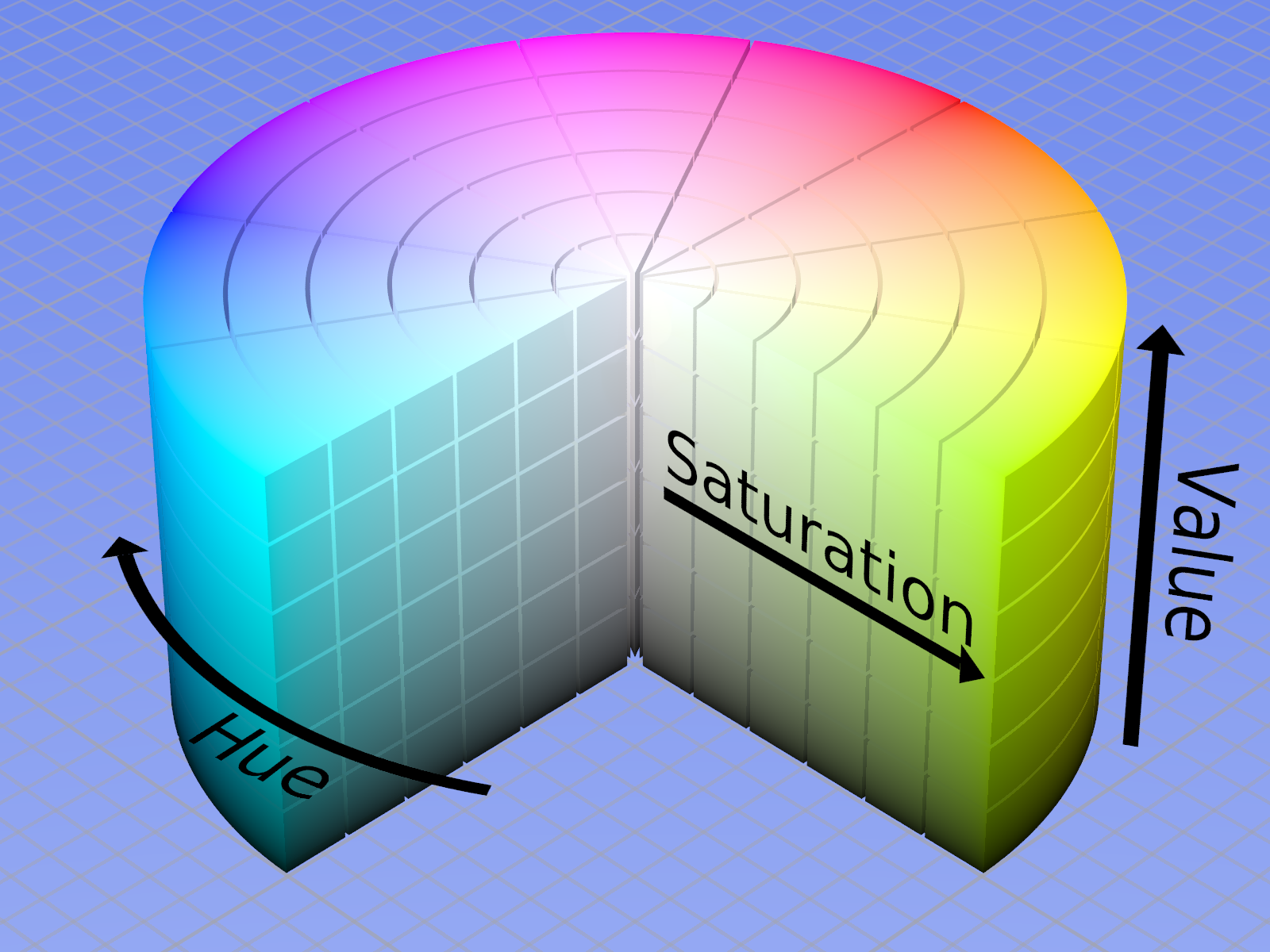
(Image source: Wikipedia and Michigan State University)

HSV representation

(Note the subtle difference between HSV and HSL)

In this setup, a color can also be represented by \[ \begin{bmatrix} H \\ S \\ V \end{bmatrix} \in \mathbb{R}^3 \] representing the Hue, Saturation, and Value, respectively.

Note that this also does not match $\mathbb{R}^3$ exactly since as the value of $H$ increases, eventually, we will come back to the same color.