Numerical algebraic geometry toolbox

Sommese & Wampler. Numerical algebraic geometry. In The mathematics of numerical analysis (Park City, UT, 1995), volume 32 of Lectures in Appl. Math., pages 749-763. Amer. Math. Soc., Providence, RI, 1996.

• Isolated and nonsingular zeros
• Witness sets for positive-dimensional components
• ...... (many many higher level data structures/algorithms)

Also, an accessible introduction:
Hauenstein & Sommese.
What is numerical algebraic geometry?
J Symb Comput 79 (2017)

Goal

"Sample" points in non-isolated components as by-products of computing isolated zero set via polyhedral homotopy method.

Repurpose waste products from polyhedral homotopy method.

Polyhedral homotopy of Huber and Sturmfels

Huber & Sturmfels. A polyhedral method for solving sparse polynomial systems. Math Comput 64, 1541-1555 (1995).

To compute all $\mathbb{C}^*$-zeros of a (Laurent) polynomial system \[ f_i(\mathbf{x}) = \sum_{\mathbf{a} \in S_i} c_{\mathbf{a}} \mathbf{x}^{\mathbf{a}} \quad\text{for } i = 1,\ldots,n \] in $\mathbf{x} = (x_1,\ldots,x_n)$, we construct $H = (h_1,\ldots,h_n)$ \[ h_i (\mathbf{x}, t) = \sum_{\mathbf{a} \in S_i} (c_{\mathbf{a}} + \color{blue}{t c_\mathbf{a}^*}) \, \mathbf{x}^{\mathbf{a}} \, \color{blue}{e^{-M \omega_{\mathbf{a}} t}}. \]

• $c_{\mathbf{a}}^*$ are generic coefficients
• $\omega_{\mathbf{a}}$ are generic rational "lifting" values
• $M > 0$ is sufficiently large

\[ f_i(\mathbf{x}) = \sum_{\mathbf{a} \in S_i} c_{\mathbf{a}} \mathbf{x}^{\mathbf{a}} \quad\longrightarrow\quad h_i (\mathbf{x}, t) = \sum_{\mathbf{a} \in S_i} (c_{\mathbf{a}} + \color{blue}{t c_\mathbf{a}^*}) \, \mathbf{x}^{\mathbf{a}} \, \color{blue}{e^{-M \omega_{\mathbf{a}} t}}. \]

• $H(\mathbf{x},t) = 0$ defines smooth "solution paths" in $(\mathbb{C}^*)^n \times (0,1)$;
• These paths escape $(\mathbb{C}^*)^n$ near the starting point $t=1$ but be approximated via "mixed cells computation" & solving binomial systems...... (can be done).
• Standard path trackers can track them from $t=1$ to $t=0$ and reach all isolated $\mathbb{C}^*$-zeros of the target system.

Polyhedral homotopy

• The number of paths equals the Bernshtein-Kushnirenko-Khovanskii (BKK) bound.
• Optimal for computing isolated $\mathbb{C}^*$-zeros of generic systems.
• Stable cell method (Huber & Sturmfels) and Random constant deformation (Li & Wang) extend this method to isolated $\mathbb{C}$-zeros.
• PHCpack, Hom4PS-*, pHom, PSS, HomotopyContinuation.jl...

Can polyhedral homotopy compute non-isolated solutions?

Non-isolated components

Zero set of a polynomial system may contain non-isolated components (i.e., positive-dimensional components).

• Non-isolated components contain infinitely many points (over $\mathbb{C}$)
• “Witness set” is the standard data structure for representing these components (Generic linear slices)

If a system has non-isolated zero component, then \[ \text{N.o. isolated zeros} \;\lneq\; \text{BKK bound} \;=\; \text{N.o. paths} \] Some paths are "wasted". (In a normal procedure)

Goal: Generate data structure like witness sets for non-isolated components from these "waste products".

A running example

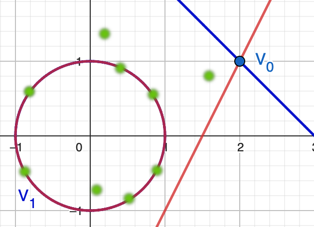
Consider the polynomial system \[ F(x_1,x_2) = \begin{bmatrix} (x_1^2 + x_2^2 - 1)(x_1 + x_2 - 3) \\ (x_1^2 + x_2^2 - 1)(2x_1 - x_2 - 3) \end{bmatrix} \]

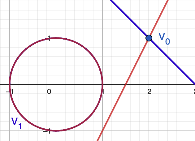
(Real picture only)

• Isolated nonsingular point $V_0$
• A (generically) reduced 1-dimensional component $V_1$
• There are singular points, which we will ignore for now

Can polyhedral homotopy method be used to compute both $V_0$ and $V_1$ from the same process?

As a parametrized system

We will write it as \[ F(x_1,x_2 \;;\; \mathbf{c}) \] where $\mathbf{c}$ is the point in $\mathbb{C}^{18}$ whose coordinates are the coefficients.

This is a family of systems parametrized by points in $\mathbb{C}^{18}$.

This is not quite right: Grassmannian is the right space for the parameters.

Zeros under perturbation

What will happen to the zero set of $F(x_1,x_2 \;;\; \mathbf{c})$ if we replace $\mathbf{c}$ by a generic point $\mathbf{c}^*$ in the coefficient space $\mathbb{C}^{18}$?

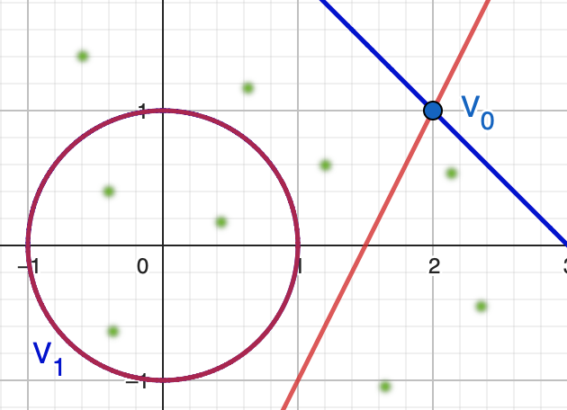
(Blurry dots are non-real zeros)

Zeros of $F(x_1,y_2 \;;\; \mathbf{c}^*)$ are isolated and nonsingular.
(All different from $V_0$ and $V_1$)

Sard's theorem: For almost all $\mathbf{c}^*$, zeros of $F(x_1,x_2 \;;\;\mathbf{c}^*)$ are isolated and nonsingular.

(Generalized Sard's Theorem) Chow, Mallet-Paret & Yorke. Finding zeroes of maps: homotopy methods that are constructive with probability one. Mathematics of Computation 32, no. 143 (1978)

Stratified perturbation

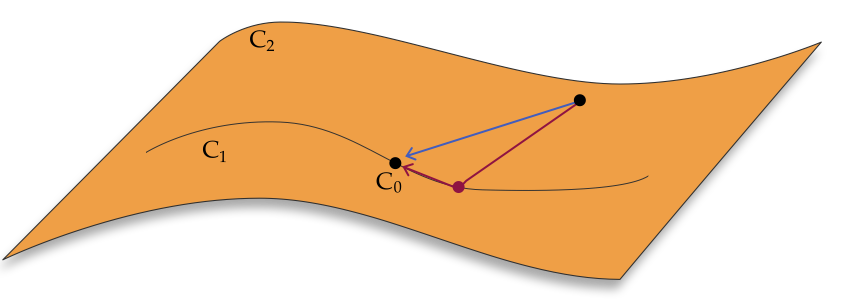
The coefficient space contains sets $C_2,C_1,C_0$ such that \[ \text{Whole parameter space} \;=\; \overline{C_2} \;\supset\; \overline{C_1} \;\supset\; \overline{C_0} \]

• $C_0 = \{ \mathbf{c} \}$ is just the original coefficient.
• $C_2$ contains almost all coefficient. For almost all $\mathbf{c}^*_2 \in C_2$, the zero set under perturbation $\mathbb{V}(F(x_1,x_2 \;;\; \mathbf{c}^*_2))$ consists of isolated and nonsingular points (Generalized Sard's theorem).
• For almost all $\mathbf{c}^*_1 \in C_1$, the zero set of $F(x_1,x_2 \;;\; \mathbf{c}^*_1)$ consists of isolated and nonsingular points, some of which are contained in $V_1$ (the 1-dimensional component of the original zero set).

Zeros at $\mathbf{c}^*_1$

For almost all $\mathbf{c}^*_1 \in C_1$, the zero set of $F(x_1,x_2 \;;\; \mathbf{c}^*_1)$ consists of 9 isolated and nonsingular points. (Blurry dots are non-real zeros)

Among them 6 points are also smooth points of $V_1$.

I.e., when perturbed coefficients $\mathbf{c}^*_1$ is restricted to $C_1$, 6 of the 9 zeros of $F(x_1,x_2 \;;\; \mathbf{c}^*)$ are "stuck" inside the component $V_1$ of the original system.

They can be used as numerically well-behaved sample points for the 1-dimensional component $V_1$ of the original system.

Sample sets

New goal: Want to compute finite "sample sets" $W_0$ and $W_1$, s.t.

• $W_0$ contains all isolated nonsingular zeros of $F$.
• $W_1$ contains some smooth points of $V_1$.

Here, a point $\mathbf{x}$ of $V_1$ is considered "smooth" if the null space of $JF(\mathbf{x})$ is 1-dimensional.

Can we compute $W_0$ and $W_1$ from the same homotopy?

Stratified polyhedral homotopy

\[ F = \begin{bmatrix} c_1\;\,x_1^3 + c_2\;\,x_2 x_1^2 + c_3\;\,x_1^2 + c_4\;\,x_2^2 x_1 + c_5\;\,x_1 + c_6\; x_2^3 + \cdots \\ c_{10} x_1^3 + c_{11} x_2 x_1^2 + c_{12} x_1^2 + c_{13} x_2^2 x_1 + c_{14} x_1 + c_{15} x_2^3 + \cdots \end{bmatrix} \]

we construct the generalized polyhedral homotopy \[ H(x_1,x_2,\color{purple}{t_1},\color{blue}{t_2}) := \begin{bmatrix} (c_1\,\,\,+ \color{purple}{t_1 c_{1}^*}\, + \color{blue}{t_2 c_1^{**}}) x_1^3 \color{blue}{e^{-M \omega_{1} t_2}} + \cdots \\ (c_{10} + \color{purple}{t_1 c_{10}^*} + \color{blue}{t_2 c_{10}^{**}}) x_1^3 \color{blue}{e^{-M \omega_{10} t_2}} + \cdots \end{bmatrix} \]

and track the 9 solution path along the parameter path \[ \begin{aligned} (1&,1) &&\longrightarrow & (1&,0) &&\longrightarrow & (0&,0) \\ &\uparrow && & &\downarrow && & &\downarrow \\ \text{Starting } &\text{points} && & &W_1 && & &W_0 \end{aligned} \]

• $W_1$: contains 6 smooth points of $V_1$ of the original system;
• $W_0$: contains all isolate nonsingular zeros of the original system;

Isolated nonsingular zeros $W_0$ and sample sets for the 1-dim component $W_1$ can be computed from the same process.

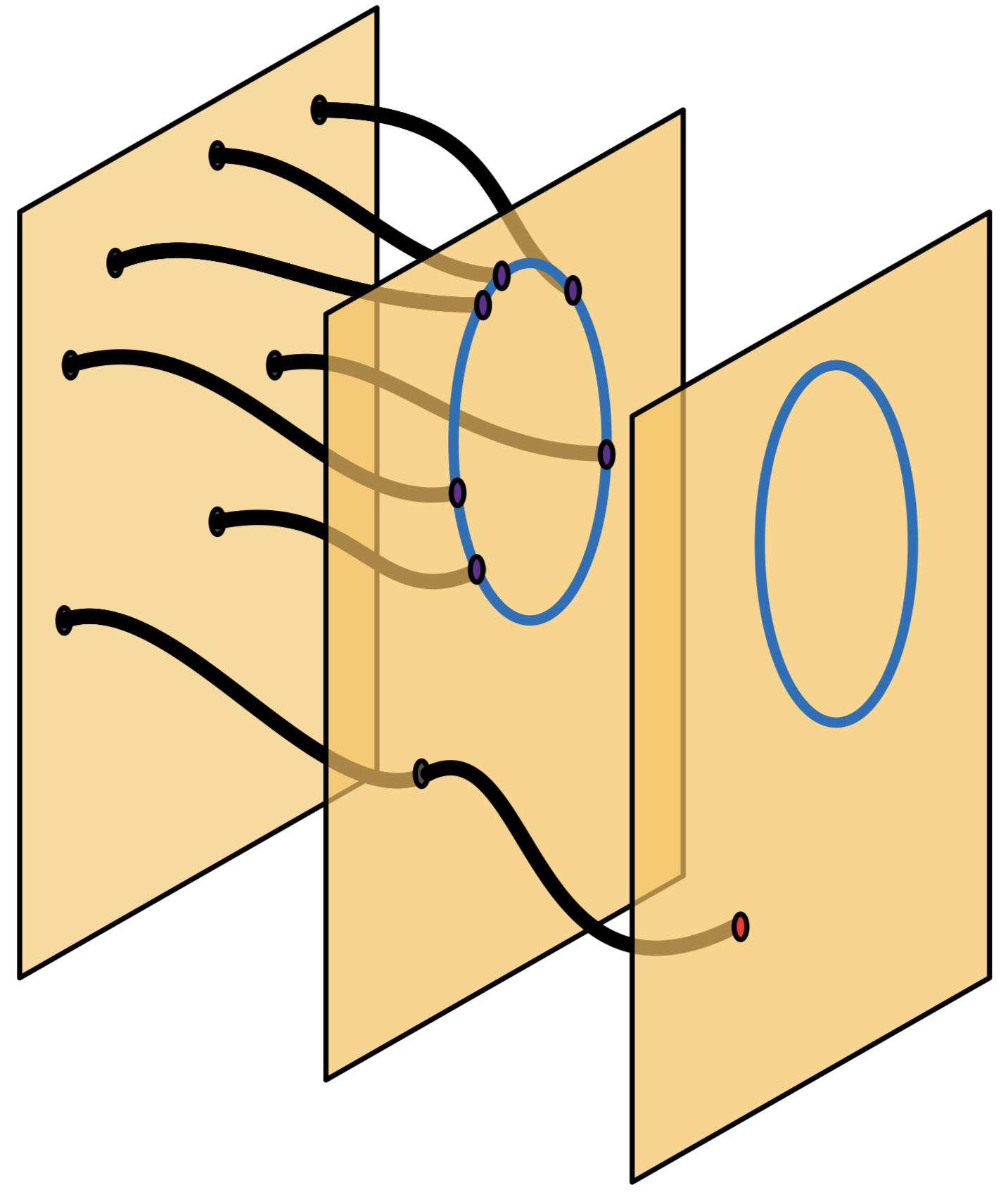
\[ \quad \quad \text{Starting points} \quad \quad W_1 \quad \quad W_0 \quad \text{(singular paths are ignored)} \]

General goal

Given a (Laurent) polynomial system $F = (f_1,\ldots,f_n)$ with \[ f_i(\mathbf{x}) = \sum_{\mathbf{a} \in S} c_{\mathbf{a}} \mathbf{x}^{\mathbf{a}} \] where $\mathbf{x} = (x_1,\ldots,x_n)$ and $S$ is their common support. We are interesting in computing the zero set of $F$ in the algebraic torus.

Stratified polyhedral homotopy

For the (Laurent) polynomial system \[ f_i(\mathbf{x}) = \sum_{\mathbf{a} \in S} c_{\mathbf{a}} \mathbf{x}^{\mathbf{a}} \] we construct the homotopy \[ h_i = \sum_{\mathbf{a} \in S} ( c_{\mathbf{a}} + \color{purple}{ t_1(s) c_{\mathbf{a}}^{(1)} + \cdots + t_n(s) c_{\mathbf{a}}^{(n)} } ) \, \mathbf{x}^{\mathbf{a}} \, \color{purple}{e^{-M \omega_{\mathbf{a}} t_n(s)}} \]

• $M > 0$ is sufficiently large, $\omega_{\mathbf{a}}$ are generic “lifting” values
• $c_{\mathbf{a}}^{(k)}$ represent a generic perturbed coefficients in $C_k$
• $(t_1(s),\ldots,t_n(s))$ gives a path in the $t$-space passing through \[ (1,\ldots,1) \to (1,\ldots,1,0) \to \cdots \to (1,0,\ldots,0) \to (0,\ldots,0) \]

Certain vertices can be skipped if we know there won't be components of certain dimensions.

$C_k$'s

Each $C_k$ is the manifold consisting of coefficient choices created by adding generic "rank-$k$" perturbation to the original coefficients: \[ \mathbf{c}_k^* = \mathbf{c} + \boldsymbol{\epsilon}_k \] if we consider them as matrices. (Better to use Grassmannian)

\[ \overline{C}_n \supset \overline{C}_{n-1} \supset \cdots \supset \overline{C}_1 \supset \overline{C}_0 = \{ \mathbf{c} \} \]

Proposition. The solution paths defined by the homotopy \[ h_i(\mathbf{x},s) = \sum_{\mathbf{a} \in S} ( c_{\mathbf{a}} + \color{purple}{ t_1(s) c_{\mathbf{a}}^{(1)} + \cdots + t_n(s) c_{\mathbf{a}}^{(n)} } ) \, \mathbf{x}^{\mathbf{a}} \, \color{purple}{e^{-M \omega_{\mathbf{a}} t_n(s)}} \] pass through the "sample sets" \[ W_{n-1} \;\to\; W_{n-2} \;\to\; \cdots \;\to\; W_0 \] at $\mathbf{t}$-values \[ (1,\ldots,1,0) \to \cdots \to (1,0,\ldots,0) \to (0,\ldots,0) \] such that

• Each $W_d$ is contained in a $d$-dimensional component;
• Each $W_d$ contains at least one point from each (generically) reduced irreducible component;
• At each point $\mathbf{x} \in W_d$ , $\operatorname{rank} JF (\mathbf{x}) = n - d$;

These sample sets can be used as numerically well-behaved representations of positive-dimensional components.

Summary

With a minor modification of how perturbation of the coefficients is done, the (unmixed) polyhedral homotopy of Huber and Sturmfels can extract "sample sets" of non-isolate (positive-dimensional) components as by-products, using wasted paths.

The number of paths to be tracked for $F = (f_1,\ldots,f_n)$ is \[ n! \operatorname{vol} ( \operatorname{conv}( \operatorname{Newt}(f_1) \,\cup\,\cdots\cup\, \operatorname{Newt}(f_n) )) \quad \text{(unmixed BKK bound)} \]

N.o. paths: Mixed vs. unmixed

\[ n! \operatorname{vol} ( \operatorname{conv}( \operatorname{Newt}(f_1) \,\cup\,\cdots\cup\, \operatorname{Newt}(f_n) )) \] Mixed volume $\longrightarrow$ volume

Easier? Volume and mixed volume computations are both #P.
(Dyer, Gritzmann, Hufnagel. On The Complexity of Computing Mixed Volumes. SIAM J Comput 27, 1998)

\[ \begin{gathered} \text{General} \\ \text{volume computation} \end{gathered} \quad\approx\quad \begin{gathered} \text{Very special} \\ \text{mixed volume computation} \end{gathered} \]

Future work

• GPU accelerated implementation: (Proof-of-concept https://arxiv.org/abs/2111.14317)
• Irreducible decomposition via monodromy?
• Computing non-reduced components?

https://www.tianranchen.org/research/papers/stratified.pdf

http://arxiv.org/abs/2108.12875 (Volume equals mixed volume)

https://arxiv.org/abs/2111.14317 (GPU acceleration)

ti@nranchen.org

Research supported, in part, by National Science Foundation, and Auburn University at Montgomery via Grant-In-Aid and Professional Improvement Leaves programs.