Oscillators

Boring example: \[ x(t) = (\cos(w \, t), \sin(w \, t)). \]

I.e., \[ \theta(t) = w \, t \] if we focus on phase angle.

Coupled oscillators

We have more interesting behavior when oscillators are coupled.

\[ \frac{d\theta}{dt} = \quad \begin{gathered} \text{One's own} \\ \text{drum beat} \end{gathered} \quad - \quad \begin{gathered} \text{Influence} \\ \text{of others} \end{gathered} \]

Two oscillators: \[ \left\{ \begin{aligned} \dot{\theta}_0 \;=\; w_0 \; - \; \text{pulling}(\theta_0,\theta_1) \\ \dot{\theta}_1 \;=\; w_1 \; - \; \text{pulling}(\theta_1,\theta_0) \end{aligned} \right. \]

This is a very naive simplification. It is a limit cycle description of "weakly coupled oscillators".

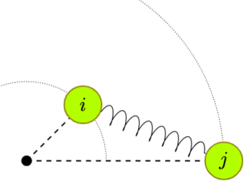
Coupling

The "pulling" should be...

• ... a function of phase difference;
• ... 0 when the phase difference is 0 or $\pi$;
• ... anti-symmetric.

These are just reasonable requirements. Certain variations deviate from these.

What about \[ \text{pulling}(\theta_i,\theta_j) = \sin(\theta_i - \theta_j) ? \] This can give rise to spontaneous synchronization (E.g., sympathetic vibration)

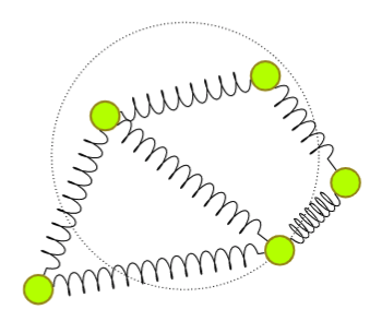
Network of coupled oscillators

We can generalize this model to networks of many oscillators coupled to one another: with \[ \frac{d\theta_i}{dt} \;= \quad \begin{gathered} \text{One's own} \\ \text{drum beat} \end{gathered} \quad - \quad \begin{gathered} \text{Influence} \\ \text{of others} \end{gathered} \] There is a long history in studying models of this form in seemingly independent fields.

• Clock synchronization
• Consensus model
• Power-flow equations
• ......

Kuramoto model

The Kuramoto model is a simple dynamical system that models the nonlinear interaction among weakly coupled oscillators.

Kuramoto. 1975, Self-entrainment of a population of coupled non-linear oscillators doi:10.1007/bfb0013365.

• Simple enough to be analyzed
• Complex enough to exhibit interesting emergent behavior

Sparsity and nonuniform coupling

More interesting cases

• The coupling strength is not uniform
• Coupling among oscillators is sparse

\[ \frac{d \theta_i}{dt} = w_i - \sum_{j \in \mathcal{N}_G(i)} k_{ij} \sin(\theta_i - \theta_j) \quad\text{for } i = 0,\ldots,n \]

• $n+1$ is the number of oscillators
• $w_i$ is the natural frequency of the $i$-th oscillator
• Symmetric coupling coefficients $k_{ij} = k_{ji} \ne 0$
• $\mathcal{N}_G(i)$ is the set of neighbors of oscillator $i$
• A connected graph $G$ encodes the network topology

Simple simulation

Synchronization

In the Kuramoto model \[ \frac{d \theta_i}{dt} = w_i - \sum_{j \in \mathcal{N}_G(i)} k_{ij} \sin(\theta_i - \theta_j) \quad\text{for } i = 0,\ldots,n \] frequency synchronization is reached when all oscillators are tuned to a common frequency (angular velocity).

• Oscillators' relative phase angle stop changing
• The dynamic picture becomes a static picture

Synchronization: a static view

A (frequency) synchronization configuration for a Kuramoto network $(G,K,w)$ is a configuration $(\theta_0,\ldots,\theta_n)$ such that \[ \frac{d \theta_0}{dt} = \frac{d \theta_1}{dt} \,=\, \cdots \, = \, \frac{d \theta_n}{dt} = c \] for some constant $c$ (synchronized frequency).

I.e., solutions to the system of equations \[ c = w_i - \sum_{j \in \mathcal{N}_G(i)} k_{ij} \sin(\theta_i - \theta_j) \quad\text{for } i = 0,\ldots,n \]

Synchronized frequency

\[ c = w_i - \sum_{j \in \mathcal{N}_G(i)} k_{ij} \sin(\theta_i - \theta_j) \quad\text{for } i = 0,\ldots,n \]

under the symmetry assumption $k_{ij} = k_{ji}$, \[ c = \frac{w_0 + \cdots + w_n}{n+1} = \overline{w} \]

I.e., the common frequency must be the mean natural frequency.

We can always normalize the network so that $\overline{w} = 0$.

And the equations become \[ 0 = w_i - \sum_{j \in \mathcal{N}_G(i)} k_{ij} \sin(\theta_i - \theta_j) \quad\text{for } i = 0,\ldots,n \]

Kuramoto equations

Synchronization configurations are exactly the solutions $(\theta_0,\ldots,\theta_n) \in [0,2\pi)^{n+1}$ to the system of equations \[ 0 = w_i - \sum_{j \in \mathcal{N}_G(i)} k_{ij} \sin(\theta_i - \theta_j) \quad\text{for } i = 0,\ldots,n \]

"Kuramoto system": $n+1$ equations in $n+1$ unknowns.

Removing redundancy

Only phase difference $\theta_i - \theta_j$ appear in \[ 0 = w_i - \sum_{j \in \mathcal{N}_G(i)} k_{ij} \sin(\theta_i - \theta_j) \quad\text{for } i = 0,\ldots,n \] so a solution remains a solution under translation. We can assume $\theta_0 = 0$. (equivalent to choosing a rotational frame of reference)

The equations are also linearly dependent: (sum to 0). So we can discard one equation: \[ 0 = w_i - \sum_{j \in \mathcal{N}_G(i)} k_{ij} \sin(\theta_i - \theta_j) \quad\text{for } i = 1,\ldots,n \] in $n$ unknowns $\theta_1,\ldots,\theta_n$: reduced Kuramoto system

Central questions

\[ 0 = w_i - \sum_{j \in \mathcal{N}_G(i)} k_{ij} \sin(\theta_i - \theta_j) \quad\text{for } i = 1,\ldots,n \]

• What is the maximum number of solutions? (Is it even finite?)
  • Lower bound: $2^n$
  • Upper bound: $\binom{2n}{n}$
  • Complication: the maximum number is topology-sensitive
• Are the solutions isolated (0-dimensional) ?

• J. Baillieul and C. Byrnes, Geometric critical point analysis of lossless power system models, IEEE Trans- actions on Circuits and Systems, 29 (1982)
• O. Coss, J. D. Hauenstein, H. Hong, and D. K. Molzahn, Locating and counting equilibria of the Kuramoto model with rank-one coupling, SIAM J. Appl. Algebra Geom., 2 (2018)
• S. Guo and F. Salam, Determining the solutions of the load flow of power systems: Theoretical results and computer implementation, 29th IEEE Conference on Decision and Control, (1990)
• J. Lindberg, A. Zachariah, N. Boston, and B. Lesieutre, The Distribution of the Number of Real Solutions to the Power Flow Equations, IEEE Transactions on Power Systems, PP (2022)
• D. K. Molzahn, D. Mehta, and M. Niemerg, Toward Topologically Based Upper Bounds on the Number of Power Flow Solutions, 2016 American Control Conference (ACC), (2016)
• ......

It's not algebraic

\[ 0 = w_i - \sum_{j \in \mathcal{N}_G(i)} k_{ij} \sin(\theta_i - \theta_j) \quad\text{for } i = 1,\ldots,n \] is not algebraic, but we can make it algebraic!

Why? Because!

Algebraic formulations

Many different ways to turn this into an algebraic system

• $s_i = \sin(\theta_i), \; c_i = \cos(\theta_i)$, and add $s_i^2 + c_i^2 = 1$;
• half-angle tangent formula
• exponential formula $x_i = e^{\mathfrak{i} \theta_i}$, then \[ \sin(\theta_i - \theta_j) = \frac{1}{2 \mathfrak{i}} \left( \frac{x_i}{x_j} - \frac{x_j}{x_i} \right) \] it produces the algebraic system \[ 0 = w_i - \sum_{j \in \mathcal{N}_G(i)} \frac{k_{ij}}{2 \mathfrak{i}} \left( \frac{x_i}{x_j} - \frac{x_j}{x_i} \right) \quad\text{for } i = 1,\ldots,n \] We prefer this one.

Laurent polynomial formulation

System of $n$ Laurent polynomial equations \[ 0 = w_i - \sum_{j \in \mathcal{N}_G(i)} \frac{k_{ij}}{2 \mathfrak{i}} \left( \frac{x_i}{x_j} - \frac{x_j}{x_i} \right) \quad\text{for } i = 1,\ldots,n \] in $n$ complex unknowns $x_1,\ldots,x_n \ne 0$ ($x_0 = 1$ is a constant).

Algebraic geometers can get to work!

• What is the maximum number of solutions? (Is it even finite?)
• Are the solutions isolated (0-dimensional) ?

A complex algebraic relaxation

\[ \begin{aligned} (\text{T}) \quad w_i &- \sum_{j \in \mathcal{N}_G(i)} k_{ij} \sin(\theta_i - \theta_j) \\ (\text{A})\quad w_i &- \sum_{j \in \mathcal{N}_G(i)} \frac{k_{ij}}{2 \mathfrak{i}} \left( \frac{x_i}{x_j} - \frac{x_j}{x_i} \right) \end{aligned} \] Every real root of (T) corresponds to a complex root of (A).

Only complex roots of (A) on the real torus $(S^1)^n$ ($|x_i| = 1$) correspond to real roots of (T). I.e., this is a relaxation can potentially introduce extraneous solutions. (A good trade-off)

Digression: 2D Toric Kumamoto problem

\[ 0 = w_i - \sum_{j \in \mathcal{N}_G(i)} \frac{k_{ij}}{2 \mathfrak{i}} \left( \frac{x_i}{x_j} - \frac{x_j}{x_i} \right) \quad\text{for } i = 1,\ldots,n \] Extraneous roots are roots outside the real torus $(S^1)^n$, i.e., roots with some $|x_i| \ne 1$.

Do they mean anything?

Digression: 2D Toric Kumamoto problem

\[ \left\{ \begin{alignedat}{5} \dot{\theta}_i = \omega_i - \sum_{j=0}^n k_{ij} \cosh(\rho_i - \rho_j) \sin(\theta_i - \theta_j) \\ \dot{\rho}_i = 0 - \sum_{j=0}^n k_{ij} \sinh(\rho_i - \rho_j) \cos(\theta_i - \theta_j) \\ \end{alignedat} \right. \;\text{for } i=1,\dots,n. \]

• $x_i = e^{-\rho_i + \mathfrak{i} \theta_i}$
• $\theta_i$ is still the phase angle
• $\rho_i = - \ln |x_i|$ measures the radial position

Central questions, relaxed

For the algebraic Kuramoto system \[ f_i(\mathbf{x}) = w_i - \sum_{j \in \mathcal{N}_G(i)} \frac{k_{ij}}{2 \mathfrak{i}} \left( \frac{x_i}{x_j} - \frac{x_j}{x_i} \right) \quad\text{for } i = 1,\ldots,n \]

• What is the maximum number of $\mathbb{C}^*$-roots? (Is it even finite?)
• Are the $\mathbb{C}^*$-roots isolated (0-dimensional) ?

If the $\mathbb{C}^*$-roots are isolated then the total number is finite, and \[ \begin{gathered} \text{Maximum} \\ \text{root count} \end{gathered} \quad=\quad \begin{gathered} \text{``Generic''} \\ \text{root count} \end{gathered} \]

Here “generic” means generic choices of parameters $w_1,\ldots,w_n$ and $k_{ij}$ (which form a Zariski closed subset of the coefficients).

Q1: Generic complex root count

Question. For generic (real or complex) natural frequencies $w_1,\ldots,w_n$ and generic but symmetric (real or complex) coupling coefficients $k_{ij} = k_{ji} \ne 0$, what is the n.o. complex solutions to \[ 0 = w_i - \sum_{j \in \mathcal{N}_G(i)} k_{ij} \left( \frac{x_i}{x_j} - \frac{x_j}{x_i} \right) \quad\text{for } i = 1,\ldots,n \; ? \]

Bernshtein’s theorem and the BKK bound

• This is the BKK bound (Bernshtein, Kushnirenko, Khovanskii)
• $\mathbb{C}^* = \mathbb{C} \setminus \{ 0 \}$, and $\mathbb{C}^*$-zeros are zeros inside $(\mathbb{C}^*)^n$
• $\operatorname{Newt}(f_i)$ is the Newton polytope of $f_i$
• $\operatorname{MV}$ is the mixed volume of $n$ convex polytopes

Bernshtein’s 2nd theorem

The converse is also true when $\operatorname{MV} > 0$.

Laurent polynomial systems satisfies this condition are said to be Bernshtein-general.

Adjacency polytope

Each edge contribute a line segment through the origin. $\mathbf{0}$ is an interior point, but still important when we consider the combinatorial features.

Equivalent to symmetric edge polytope studied in other fields. (See, e.g. D'Alì, Delucchi, Michałek. Many Faces of Symmetric Edge Polytopes. Electron J Comb 29, 2022)

Adjacency polytope and Newton polytopes

The algebraic Kuramoto system \[ f_i(\mathbf{x}) = w_i - \sum_{j \in \mathcal{N}_G(i)} k_{ij} \left( \frac{x_i}{x_j} - \frac{x_j}{x_i} \right) \quad\text{for } i = 1,\ldots,n, \] involves constant terms and monomials $x_i / x_j$ for $\{ i, j \} \in E$. Therefore, \[ \begin{aligned} \nabla_G &:= \{ \mathbf{0} \} \cup \{ \pm (\mathbf{e}_i - \mathbf{e}_j) \mid \{ i, j \} \in E \} \\ &= \operatorname{Supp}(f_i) \; \cup \, \cdots \, \cup \; \operatorname{Supp}(f_n) \end{aligned} \]

It is the Newton polytope of the randomization $R \cdot F(\mathbf{x})$ for a square matrix $R$ (random linear combinations): \[ \nabla_G = \operatorname{Newt}( R \cdot F ) \]

Adjacency polytope bound

This is the adjacency polytope bound.

\[ \begin{gathered} \text{Generic} \\ \mathbb{C}\text{-root count} \end{gathered} \quad\le\quad \begin{gathered} \text{Adjacency} \\ \text{polytope bound} \\ \end{gathered} \]

Why adjacency polytope ?

We know much about $\nabla_G := \{ \mathbf{0} \} \cup \{ \pm (\mathbf{e}_i - \mathbf{e}_j) \mid \{ i, j \} \in E \}$

• Higashitani, Jochemko, Michałek. Arithmetic aspects of symmetric edge polytopes. Mathematika 65, 2019.
• Chen, Davis, Korchevskaia. Facets and facet subgraphs of adjacency polytopes. Arxiv 2021.

A series of relaxations

For the algebraic Kuramoto system \[ f_i(\mathbf{x}) = w_i - \sum_{j \in \mathcal{N}_G(i)} k_{ij} \left( \frac{x_i}{x_j} - \frac{x_j}{x_i} \right) \quad\text{for } i = 1,\ldots,n \] with parameters $w_1,\ldots,w_n$ (natural frequencies) and symmetric coupling coefficients $k_{ij} = k_{ji}$, \[ \begin{gathered} \text{Real} \\ \text{(isolated)} \\ \text{root count} \end{gathered} \;\le\; \begin{gathered} \text{Generic} \\ \mathbb{C}\text{-root} \\ \text{count} \end{gathered} \;\le\; \begin{gathered} \text{BKK} \\ \text{bound} \end{gathered} \;\le\; \begin{gathered} \text{Adjacency} \\ \text{polytope} \\ \text{bound} \\ \end{gathered} \]

A reasonable conjecture

\[ \begin{gathered} \text{Generic} \\ \mathbb{C}\text{-root} \\ \text{count} \end{gathered} \;=\;\; \begin{gathered} \text{BKK} \\ \text{bound} \end{gathered} \;\;=\; \begin{gathered} \text{Adjacency} \\ \text{polytope} \\ \text{bound} \\ \end{gathered} \]

Generic root count result

\[ \begin{gathered} \text{Generic} \\ \mathbb{C}\text{-root} \\ \text{count} \end{gathered} \;=\;\; \begin{gathered} \text{BKK} \\ \text{bound} \end{gathered} \;\;=\; \begin{gathered} \text{Adjacency} \\ \text{polytope} \\ \text{bound} \\ \end{gathered} \]

Obstacles

\[ f(\mathbf{x}) = w_i - \sum_{j \in \mathcal{N}_G(i)} \frac{k_{ij}}{2 \mathbf{i}} \left( \frac{x_i}{x_j} - \frac{x_j}{x_i} \right) \quad\text{for } i = 1,\ldots,n \]

1. In each polynomial, the monomials $x_i/x_j$ and $x_j/x_i$, must share the same coefficient $\frac{k_{ij}}{2 \mathbf{i}}$.
2. For any edge $\{i,j\} \in E$, the $i$-th and $j$-th polynomial always have the terms $\frac{k_{ij}}{2\mathbf{i}} (x_i x_j^{-1} - x_j x_i^{-1})$ and $\frac{k_{ji}}{2\mathbf{i}} (x_j x_i^{-1} - x_i x_j^{-1})$.
3. Unless $G$ is the complete graph, the Newton polytopes are not all full-dimensional.

How to prove this?

There are many ways. We followed a familiar recipe

1. Construct a homotopy
2. Prove smoothness
3. Count the number of homotopy paths

A nonlinear homotopy

Basing on \[ f_i(\mathbf{x}) = w_i - \sum_{j \in \mathcal{N}_G(i)} \frac{k_{ij}}{2 \mathbf{i}} \left( \frac{x_i}{x_j} - \frac{x_j}{x_i} \right) \quad\text{for } i = 1,\ldots,n \] we define $H(\mathbf{x},t) = (h_1,\ldots,h_n)$ \[ h_i (\mathbf{x},t) = w_i - \sum_{j \in \mathcal{N}_G(i)} \frac{k_{ij}}{2 \mathfrak{i}} \; t^{\alpha_{ij}} \; \left( \frac{x_i}{x_j} - \frac{x_j}{x_i} \right) \quad\text{for } i = 1, \ldots,n \] with generic but symmetric rational “lifting” values $\alpha_{ij} = \alpha_{ji} \approx 1$.

Structure preserving polyhedral homotopy

\[ h_i := w_i - \sum_{j \in \mathcal{N}_G(i)} \frac{k_{ij}}{2 \mathfrak{i}} \; t^{\alpha_{ij}} \; \left( \frac{x_i}{x_j} - \frac{x_j}{x_i} \right) \;\text{for } i = 1, \ldots,n \] with generic but symmetric rational “lifting” values $\alpha_{ij} = \alpha_{ji} \approx 1$. defines a structure preserving polyhedral homotopy (Huber & Sturmfels. A polyhedral method for solving sparse polynomial systems. Math Comput 64, 1541-1555, 1995)

• At $t=1$, $h_i(\mathbf{x},1) \equiv f_i(\mathbf{x})$
• Each $h_i (\mathbf{x}, t)$ is holomorphic in $\mathbf{x}$ and $t$ away from $t=0$
• For any $t \ne 0$, symmetry in the coefficients is preserved \[ \frac{k_{ij}}{2 \mathfrak{i}} t^{\alpha_{ij}} = \frac{k_{ji}}{2 \mathfrak{i}} t^{\alpha_{ji}} \]

Homotopy paths

\[ 0 = h_i = w_i - \sum_{j \in \mathcal{N}_G(i)} \frac{k_{ij}}{2 \mathfrak{i}} \; t^{\alpha_{ij}} \; \left( \frac{x_i}{x_j} - \frac{x_j}{x_i} \right) \] for $i = 1, \ldots,n$ defines smooth homotopy paths over $t \in (0,1]$.

Under the assumption that $k_{ij}$'s and $w_i$'s are chosen generically, \[ \text{N.o. paths} \;=\; \text{Generic root count} \] So the root counting question becomes a path counting question.

Side note: the tropical view

Half of the question is tropical: Going back to \[ f_i(\mathbf{x}) = w_i - \sum_{j \in \mathcal{N}_G(i)} \frac{k_{ij}}{2 \mathbf{i}} \left( \frac{x_i}{x_j} - \frac{x_j}{x_i} \right) \quad\text{for } i = 1,\ldots,n \] We assign the symmetry preserving valuations \[ \begin{aligned} \operatorname{val}(w_i) &= 0 &&\text{and} & \operatorname{val}(k_{ij}) &= \operatorname{val}(k_{ji}) = \alpha_{ij} \end{aligned} \]

What is the intersection number of the $n$ tropical hypersurfaces \[ \mathbb{V}(\;\operatorname{Trop}(f_1) \;) \;\cap\; \cdots \;\cap\; \mathbb{V}(\;\operatorname{Trop}(f_n) \;) \]

This is the tropical version of the generic root count question.

Randomization

For a square algebraic system $F = (f_1,\ldots,f_n)$, analysis can be simplified through "randomization" (random linear combinations): For any $n \times n$ nonsingular matrix $R$, \[ F(\mathbf{x}) \quad\quad\text{and}\quad\quad R \cdot F(\mathbf{x}) \] have the same zero set. So we can study the "randomized Kuramoto system" $R \cdot F(\mathbf{x})$ instead.

• all polynomials in $R \cdot F (\mathbf{x})$ involve all monomials;
• the Newton polytopes are all identical (unmixed case);

Terminology: Numerical analysts would call $F \mapsto R \cdot F$ "preconditioning" (a standard practice to improve the numerical condition of systems of equations).

Digression: Why randomize?

Randomization turns a mixed system to an unmixed system (every polynomial involves every monomial).

• Tropical intersection $\to$ Stable self-intersection
• Fine mixed subdivision $\to$ Triangulation
• Mixed volume computation $\to$ volume computation

Easier? Volume and mixed volume computations are both #P.

(Dyer, Gritzmann, Hufnagel. On The Complexity of Computing Mixed Volumes. SIAM J Comput 27, 1998)

Digression: Mixed volume vs. volume

The specialized problem of computing mixed volume of simplices is at least as "hard" as the general problem of computing volume. (http://arxiv.org/abs/2108.12875)

\[ \begin{gathered} \text{General} \\ \text{volume computation} \end{gathered} \quad\approx\quad \begin{gathered} \text{Very special} \\ \text{mixed volume computation} \end{gathered} \]

Back to path counting

We want to count the number of paths over $t \in (0,1]$ defined by \[ 0 = h_i = w_i - \sum_{j \in \mathcal{N}_G(i)} \frac{k_{ij}}{2 \mathfrak{i}} \; t^{\alpha_{ij}} \; \left( \frac{x_i}{x_j} - \frac{x_j}{x_i} \right) \;\text{for } i = 1, \ldots,n. \]

It's much easier to count paths defined by the randomized version \[ H^* := R \cdot H = 0 \] for a generic (nonsingular) square matrix $R$.

The stable self-intersections "points" of $\operatorname{Trop}(H^*)$ are in 1-to-1 correspondence with cells in a unimodular triangulation of $\partial \nabla_G$. And the total number is exactly $\operatorname{Vol}(\nabla_G)$.

Stable self intersection

There are exactly $\operatorname{Vol}(\nabla_G)$ stable self-intersections of $\operatorname{Trop}(H^*)$.

Each gives rise to a single path defined by the structure preserving polyhedral homotopy \[ 0 = h_i = w_i - \sum_{j \in \mathcal{N}_G(i)} \frac{k_{ij}}{2 \mathfrak{i}} \; t^{\alpha_{ij}} \; \left( \frac{x_i}{x_j} - \frac{x_j}{x_i} \right) \;\text{for } i = 1, \ldots,n. \]

Therefore \[ \operatorname{Vol}(\nabla_G) \;\le\; \begin{gathered} \text{N. o.} \\ \text{paths} \end{gathered} \;=\; \begin{gathered} \text{Generic} \\ \text{root count} \end{gathered} \;\le\; \operatorname{Vol}(\nabla_G) \]

Bernshtein-generalness

\[ \begin{gathered} \text{Generic} \\ \mathbb{C}\text{-root} \\ \text{count} \end{gathered} \;=\;\; \begin{gathered} \text{Adjacency} \\ \text{polytope} \\ \text{bound} \\ \end{gathered} \]

We also know that \[ \begin{gathered} \text{Generic} \\ \mathbb{C}\text{-root} \\ \text{count} \end{gathered} \le \begin{gathered} \text{BKK} \\ \text{bound} \end{gathered} \le \begin{gathered} \text{Adjacency} \\ \text{polytope} \\ \text{bound} \\ \end{gathered} \] So they must be all equal, and the algebraic Kuramoto system is Bernshtein-general.

Recap: Generic root count

\[ \begin{gathered} \text{Generic} \\ \mathbb{C}\text{-root} \\ \text{count} \end{gathered} \;=\;\; \begin{gathered} \text{BKK} \\ \text{bound} \end{gathered} \;\;=\; \begin{gathered} \text{Adjacency} \\ \text{polytope} \\ \text{bound} \\ \end{gathered} \]

Computational implications

\[ \text{Generic } \mathbb{C}\text{-roots} \;=\; \text{A.P. bound} \]

The structure preserving polyhedral homotopy is an optimal homotopy method for solving algebraic Kuramoto equations...

... IF $\mathbb{C}$-roots are needed.

This vs. the original polyhedral homotopy

Differences:

• Use symmetric lifting values ($\operatorname{val}(k_{ij}) = \operatorname{val}(k_{ji})$)
• Different start system

Non-generic situations

\[ \begin{gathered} \text{Generic} \\ \mathbb{C}\text{-root} \\ \text{count} \end{gathered} \;\;=\; \begin{gathered} \text{Adjacency} \\ \text{polytope} \\ \text{bound} \\ \end{gathered} \]

• when will the actual root count drop below generic root count?
• by how much?

Missing roots: Exceptional couplings

Q2: Under the assumption of generic $w$'s, what are the choices of coupling coefficients $k_{ij}$'s for which \[ \text{Actual $\mathbb{C}$-root count} \; < \; \text{Generic $\mathbb{C}$-root count} \]

This set is the exceptional coupling coefficients.

Cycle basis description

There are a few variations based on graph topology.

General description

Example: 4-cycle

There are 4 coupling coefficients $k_{01},k_{12},k_{23},k_{30} \ne 0$

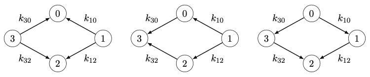
Refined root count for $C_4$

Root count drops below the generic root count if and only if \[ \begin{aligned} \frac{ k_{01} k_{12} }{ k_{23} k_{30} } &= 1 &&\text{or} & \frac{ k_{01} k_{30} }{ k_{12} k_{23} } &= 1 &&\text{or} & \frac{ k_{01} k_{23} }{ k_{12} k_{30} } &= 1 \end{aligned} \]

By how much?

• Only 1 out of 3 holds: 10 roots (missing 2), and all can be real
• Only 2 out of 3 hold: 8 roots (missing 4), and all can be real
• All 3 holds: 6 roots (missing 6), and all can be real

Balanced subnetwork

Balanced subnetworks always come in transpose pairs.

\[ \begin{aligned} \frac{ k_{01} k_{12} }{ k_{23} k_{30} } &= 1 &&\text{or} & \frac{ k_{01} k_{30} }{ k_{12} k_{23} } &= 1 &&\text{or} & \frac{ k_{01} k_{23} }{ k_{12} k_{30} } &= 1 \end{aligned} \]

Each max. balance subnetwork is -1 root

With this we can rephrase: For the $C_4$ network (with generic natural frequencies), \[ \begin{gathered} \text{Actual} \\ \text{root} \\ \text{count} \end{gathered} \quad = \quad \begin{gathered} \text{Generic} \\ \text{root} \\ \text{count} \end{gathered} \quad - \quad \begin{gathered} \text{N. o. maximum } \\ \text{balanced} \\ \text{subnetwork} \end{gathered} \]

Example: 6-cycle case

Generic root count: 60

• Choosing \[ [ k_{01}, k_{12}, k_{23}, k_{34}, k_{45}, k_{50} ] = [ \pm 1, \pm 1, \pm 1, \pm 1, \pm 1, \pm 1 ] \] with an odd number of negative choices, then there will be 20 max. balanced subetworks (10 transpose pairs), and \[ \text{Root count} \;=\; 60 - 20 \;=\; 40 \]
• Choosing \[ [ k_{01}, k_{12}, k_{23}, k_{34}, k_{45}, k_{50} ] = [ \pm s, \pm s, \pm t, \pm t, \pm t, \pm t ] \] with an odd number of negative choices and $s \ne t$, then there will be 12 max. balanced subnetworks (12 transpose pairs), and \[ \text{Root count} \;=\; 60 - 12 \;=\; 48 \]

Refined root count unicycle network

Future directions

• Refined root count for networks beyond unicycle networks
• Investigation of max. real root count vs. A. P. bound
• Formula for A. P. bound for all networks
• A graph theoretical method for enumerating cells in a unimodular triangulation of the A. P. $\nabla_G$.

Non-isolated solution sets

Another way generic root count is broken: appearance of non-isolated (positive-dimensional) components. They represent synchronization configurations with at least one degree of freedom.

• (Complete graphs) P. Ashwin, C. Bick, and O. Burylko. Identical Phase Oscillator Networks: Bifurcations, Symmetry and Reversibility for Generalized Coupling, Frontiers in Applied Mathematics and Statistics, 2 (2016)
• (Complete graphs) O. Coss, J. D. Hauenstein, H. Hong, and D. K. Molzahn. Locating and counting equilibria of the Kuramoto model with rank-one coupling, SIAM J. Appl. Algebra Geom., 2 (2018)
• (Complete graphs and cycles) J. Lindberg, A. Zachariah, N. Boston, and B. Lesieutre. The Distribution of the Number of Real Solutions to the Power Flow Equations. IEEE Transactions on Power Systems, PP (2022)
• D. Sclosa, Kuramoto networks with infinitely many stable equilibria. (2022)

Constructing positive-dimensional solutions

Indeed we can construct a $\mathbb{C}^*$-orbit \begin{align*} \begin{bmatrix} x_1(\lambda) & \cdots & x_m(\lambda) \end{bmatrix} &= ( \lambda \cdot \boldsymbol{\eta}_{\vec{T}} \circ (\mathbf{k}(\vec{T})^{-I}) )^{Q(\vec{T})^{-1}} \\ x_i &= \pm x_{\pi(i)} \quad\text{for } i = m+1, \ldots, n, \end{align*}

(Require further explanation) Main point: It contain an 1-dimensional orbit parametrized by a system of Laurent monomials.

Real-orbits

The original Kuramoto equations will have positive-dimensional real solution components.

For the 4-cycle example, when the natural frequencies are identical, and $k_{ij}$'s are identical, we have 1-dimensional solution sets \[ \left\{ \begin{aligned} \theta_0 &= 0 \\ \theta_1 &= t + \pi + \sigma^{10} \\ \theta_2 &= \pi + \sigma^{12}_{10} \\ \theta_3 &= t + \sigma^{30} \\ \end{aligned} \right. \quad \left\{ \begin{aligned} \theta_0 &= 0 \\ \theta_1 &= \sigma^{10} + t \\ \theta_2 &= \pi + \sigma^{21}_{10} \\ \theta_3 &= \sigma^{30} - t \end{aligned} \right. \quad \left\{ \begin{aligned} \theta_0 &= 0 \\ \theta_1 &= \sigma^{10} - t \\ \theta_2 &= \sigma^{21}_{10} -2t \\ %\sigma(k_{21}/k_{10}) \\ \theta_3 &= \pi + \sigma^{30} -t \\ \end{aligned} \right. \] $\sigma$'s are phase shift values, $0$ or $\pi$, that only used to adjust for the signs of $k_{ij}$'s (not very important).

Beyond unicycle networks

There is a similar $\mathbb{C}^*$-orbit formula that parametrizes an 1-dimensional orbit inside the zero set.

Example: 2 cycles sharing an edge

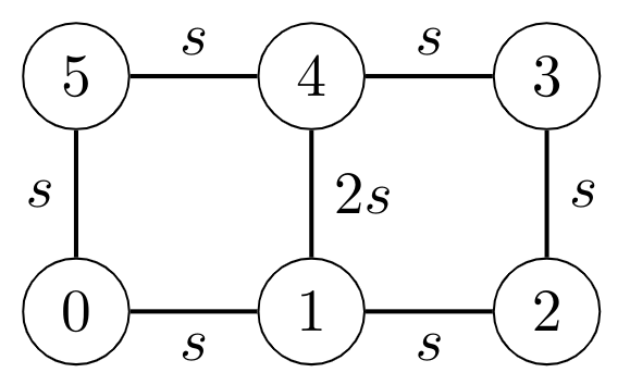
The construction produces the 1-dimensional real solution set \[ (\theta_0,\theta_1,\theta_2,\theta_3,\theta_4,\theta_5) = ( 0, t + \pi, 0, t, \pi, t ) \] This is one of many real orbits.

Observation: The positive-dimensional solution sets constructed this way are actually solution set of certain initial systems!

https://www.tianranchen.org/research/papers/krootcount.pdf

https://arxiv.org/abs/2107.12315

http://arxiv.org/abs/2108.12875

Research supported, in part, by National Science Foundation, and Auburn University at Montgomery via Grant-In-Aid program, PIL program, and undergraduate research experience program.